Operators

Algebraic operators

Note

Let’s assume that in this section we will adress the possible types of operands as several domains of values with the following convention:

iv : Integer value
rv : Real value
ii : Integer Interval
ri : Real Interval
ie : Integer Enumeration
re : Real Enumeration

An algebraïc operator is an operator on numerical operands.

Unary algebraic operators

operator	operand	meaning
sin	rv, iv, ri, ii, de, ie	sinus
cos	rv, iv, ri, ii, de, ie	cosinus
tan	rv, iv, ri, ii, de, ie	tangent
asin	rv, iv, ri, ii, de, ie	arc sinus
acos	rv, iv, ri, ii, de, ie	arc cosinus
atan	rv, iv, ri, ii, de, ie	arc tangent
sinh	rv, iv, ri, ii, de, ie	hyperbolic sinus
cosh	rv, iv, ri, ii, de, ie	hyperblic cosinus
tanh	rv, iv, ri, ii, de, ie	hyperbolic tangent
asinh	rv, iv, ri, ii, de, ie	hyperbolic arc sinus
acosh	rv, iv, ri, ii, de, ie	hyperbolic arc cosinus
atanh	rv, iv, ri, ii, de, ie	hyperbolic arc tangent
ln	rv, iv, ri, ii, de, ie	neperian logarithm
exp	rv, iv, ri, ii, de, ie	exponential
abs	rv, iv, ri, ii, de, ie	absolute value
sqr	rv, iv, ri, ii, de, ie	square
sqrt	rv, iv, ri, ii, de, ie	square root
trunc	rv, iv, ri, ii, de, ie	truncature

The syntax is the following one:

with op in {sin, cos, tan, asin, acos, atan, sinh, cosh, tanh, asinh, acosh, atanh, ln, exp, abs, sqrt}

op(<expr>)

Binary algebraic operators

operator	operand	meaning
+	rv, iv, ri, ii, de, ie	addition
-	rv, iv, ri, ii, de, ie	difference
*	rv, iv, ri, ii, de, ie	multiplication
/	rv, iv, ri, ii, de, ie	division
^	rv, iv, ri, ii, de, ie	power
min	rv, iv, ri, ii, de, ie	minimum
max	rv, iv, ri, ii, de, ie	maximum

The syntax is the following one:

 with op in {+, -, *, /, ^}

 <expr1> op <expr2>

with op in {min, max}

 op(<expr1> , <expr2>)

Boolean operators

Boolean operators are operators on Boolean operands.

Unary boolean operators

operator	operand	meaning
not	iv in {0,1}, ii in [0,1], ie in {0,1}	boolean negation

The syntax is the following one:

not(<expr>)

Binary boolean operators

operator	operand	meaning
or	iv in {0,1}, ii in [0,1], ie in {0,1}	boolean or
and	iv in {0,1}, ii in [0,1], ie in {0,1}	boolean and

The syntax is the following one:

with op in {or, and}

<expr1> op <expr2>

Piecewise operators

It may be necessary in some design problems to express piecewise functions from R to R. This is the case when a function is defined continuously by pieces.

Piecewise operators can be linear or nonlinear.

For nonlinear piecewise operator the syntax is the following one:

Let’s assume that we want to model in DEPS the following piecewise function:

\(y = f(x)\) defined on [0, 100] such that:

\(f(x) = x\) if \(x\) ∈ [0, 1]

\(f(x)=x^3\) if \(x\) ∈ [1, 10]

\(f(x) = 1e^2/x\) if \(x\) ∈ [10, 100]

Model PieceWiseEx()
Constants
Variables
x : Real;
y : Real;
Elements
Properties
y = pw(x, [0,1], x^3, [1, 10], x^3, [10, 100], 1e2/x);
End

For linear piecewise operator, the syntax is the following ones:

pwl(<varg>, <TableName>);

pwl(<varg>, (varg1, vim1), (varg2, vim2), …, (vargn, vimn));

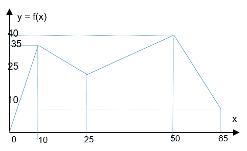
Let’s assume that we want to model in DEPS the following piecewise function:

Two ways are possible:

On the one hand, we can put the breacking points in a table and use the pwl operator as follow:

Table PwlValues
Attributes
x  :  Real;
y  :  Real;
Tuples
[0, 0],
[10, 35] ,
[25, 25],
[50, 40],
[65, 10]
End

Model PieceWiseEx()
Constants
Variables
x : Real;
y : Real;
Elements
Properties
y = pw(x, PwlValues);
End

On the other hand, we can put the breacking points inside the pwl operator as folllow:

Model PieceWiseLinEx()
Constants
Variables
x : Real;
y : Real;
Elements
Properties
y = pwl(x, (0, 0), (10, 35), (25, 25), (50, 40), (65, 10));
End